
How to Dynamically Filter in Jet Reports Using a Drop Down-List

This blog provides step-by step instructions on how to create a dropdown list for end users to use to filter a Jet Report without the end user needing Jet Reports license.
As a report designer, when working with Jet Global’s Jet Reports, it can be time consuming to create multiple versions of the same report with only one filter value changed in each version. You can use Microsoft Excel’s drop-down list feature to create a dynamic filter for end users to use on a Jet Report so that you don’t have to create multiple versions of the same report.
In this example, you will create a report showing regional sales and you want to be able to allow the end user filter on the sales representative. The end user in this case doesn’t have a Jet license, so they can’t update Jet formulas or refresh the report themselves. You will need to create a hidden sheet with the data for all of the filter options and then reference the data from that hidden sheet on the main report page using a VLOOKUP function for the filter to work.
To create this report:
- Create a new Jet Report Excel worksheet.
- Add a sheet for the hidden data. Make sure you use auto+hide+value+hidesheet in cell A1 so the sheet will remain hidden. Alternatively, you can add +lock to the list of keywords in A1 if you plan on password protecting the report.Figure 1 – Jet Reports A1 keywords for hidden sheet
- On your hidden sheet, create a table or rows and columns (you can even use Jet replicating rows) of the data you want your final report to pull. Make sure your columns are the values you want to filter on. In this example, the final report will allow the end user to filter on the name of the sales rep, so the names are the column headers.
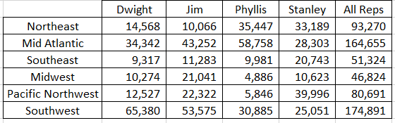
Figure 2 – Create data table on hidden sheet - Still on your hidden sheet, create a second table or chart containing two columns to list the filter options you want. In the first column, list the filters in the order you want them displayed.
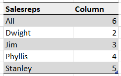
Figure 3 – Create a two-column table for filter options In the second column of the table you will list the column numbers that correspond to the filter values from the first data table you created in Step 3. The column numbers in column 2 of the table will be used for a VLOOKUP function in step 10. (You can go here for more information on creating a table in Excel.)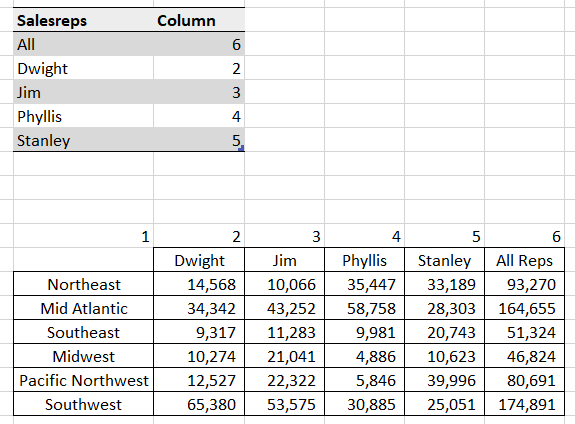
Figure 4 – Corresponding column numbers between the filter table and the data table on hidden sheet - Create a second tab in the workbook for the report you want the end users to see. Add auto+hide+values to cell A1 on the new tab. Note: Do not use +lock keyword on this tab or your end users will be unable to use the dropdown filter.
- Near the top of your report, select a cell to be used as the filter dropdown. While that cell is highlighted, go to the Data section at the top of the Excel ribbon and select the Data Validation button to create a dropdown filter.

Figure 5 – Microsoft Excel Data Validation - In the Data Validation window, set the Allow field to List, select the boxes for Ignore blank and In-cell dropdown. Then in the Source field, select the column from the table you created on the hidden sheet that has the list of filters you want the end users to use.
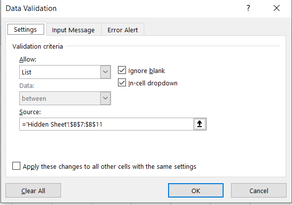
Figure 6 – Microsoft Excel Data Validation settings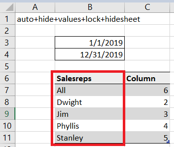
Figure 7 – Microsoft Excel dropdown filters column selection - Still in the Data Validation window, click the Input Message tab to enter text to be displayed when an end user selects the filter cell.
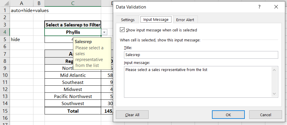
Figure 8 – Microsoft Excel Data Validation Input Message - Finally, select the Error Alert tab in the Data Validation window to enter an optional error message if a user were to try to input something in the filter cell instead of using the dropdown filter. Click OK when finished.
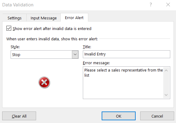
Figure 9 – Microsoft Excel Data Validation Error Alert - In the cell below your newly created filter cell, enter a VLOOKUP formula to look at the filter option selected and reference the table built in Step 4 on the hidden sheet to retrieve the column number of the data from the data on the hidden sheet. (You can go here for more information on the VLOOKUP formula in Excel.
= VLOOKUP(cell reference for dropdown filter, cell reference for table on hidden sheet, column #2, FALSE for an exact match)
Example:
=VLOOKUP(C4, Table 1, 2, FALSE)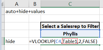
Figure 10 – Microsoft Excel VLOOKUP formula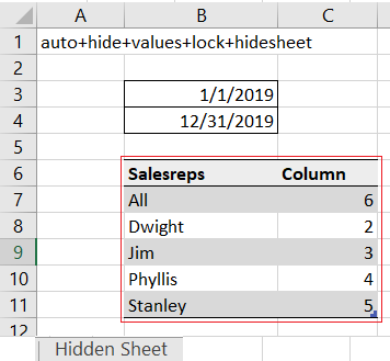
Figure 11 – Microsoft Excel VLOOKUP formula table referenceThe result of the VLOOKUP formula should be the column number of the selected filter option from the hidden sheet.
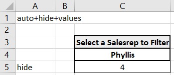
Figure 12 – Microsoft Excel VLOOKUP result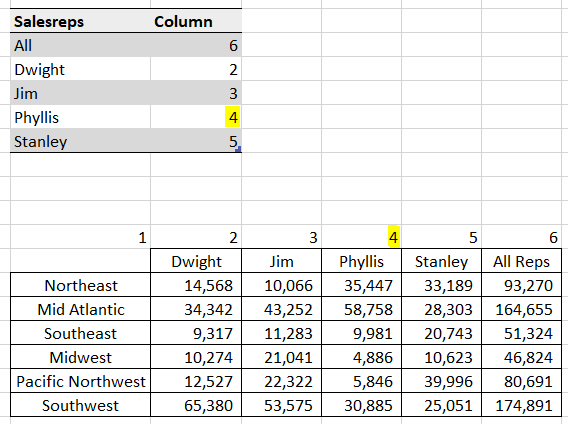
Figure 13 – Column numbers matching between VLOOKUP, filtering table, and data table - Hide the row for your VLOOKUP formula using the Jet keyword “hide” in column A of the row.
- On the tab of the worksheet that your end users will see, you can now build the report to which you want to apply the dropdown filter. Use the VLOOKUP function for your report values by using the hidden column reference for the column number input in the VLOOKUP formula.
= VLOOKUP(cell reference for category, cell reference for data chart on hidden sheet, cell reference for column number, FALSE for an exact match)
Example:
=VLOOKUP(C9, ‘Hidden Sheet’!$B$16:$G$22,$C$5,FALSE)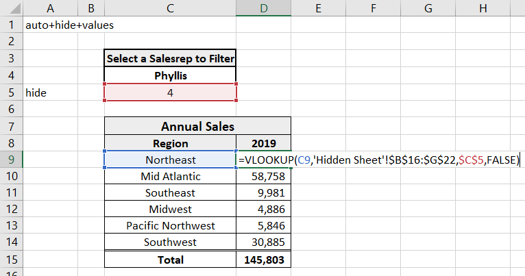
Figure 14 – Microsoft Excel VLOOKUP column number cell referenceBuild out the report you want your end users to see and be able to filter, run your Jet report so it is no longer in Design mode, and you are ready to share the report for end users to filter.
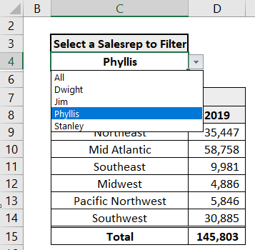
Figure 15 – Jet Reports dropdown filter available for end users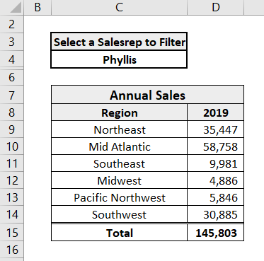
Figure 16 – Jet Reports dropdown filter applied by end user
If you have any questions about Jet Global, Jet Reports, or other Dynamics 365 Business Central or NAV questions for any version, contact ArcherPoint.
Read more “How To” blogs from ArcherPoint for practical advice on using Microsoft Dynamics 365 Business Central or NAV.
Trending Posts
- Login Error: Communication protocol mismatch between client and server
- How to Make Measures Total Correctly in Power BI Tables
- The Microsoft Technology Stack – What Is It & Why Should You Care?
- MRP vs. MPS: Choosing the Right Planning Approach for Your Manufacturing Business
- Guide to How Manufacturers Can Implement Quality Control Systems Using Business Central
Stay Informed
Subscribe to Communications
"*required" indicates required fields